Over the weekend, I decided to play around with a simplified version of a federated Q-learning algorithm. Inspired by recent research on Fed-DVR-Q, I built a small simulation where multiple agents learn to navigate a maze using Q-learning. The twist? The agents share their learned Q-tables periodically—mimicking intermittent communication in a federated learning setup.
In this post, I’ll walk you through the code step by step, explain each block in detail, and describe the outputs I observed.
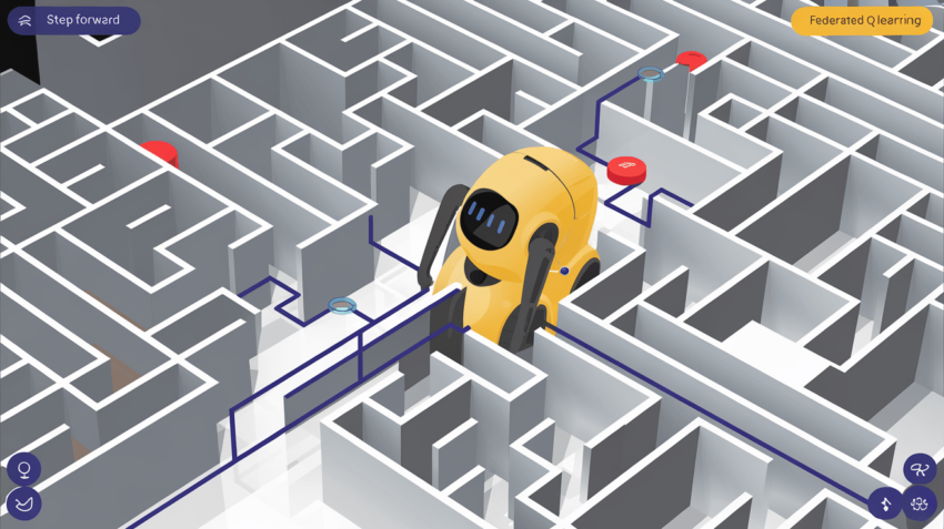
The maze is defined as a 5×5 grid where: – 0 represents a free cell. 1 represents a wall. The starting cell is (0, 0) and the goal (treasure) is at (4, 4). An agent receives a reward of –1 for each step (to encourage shorter paths) and +10 when it reaches the goal.
1. Defining the Maze Environment
python
# ---------- Maze Environment Definition ----------
import numpy as np
import matplotlib.pyplot as plt
import random
import time

# Our maze: a 5x5 grid where 0 is free and 1 is a wall.
maze = np.array([
    [0, 1, 0, 0, 0],
    [0, 1, 0, 1, 0],
    [0, 0, 0, 1, 0],
    [0, 1, 1, 1, 0],
    [0, 0, 0, 0, 0]
])
rows, cols = maze.shape
start = (0, 0)   # starting position (row, col)
goal = (4, 4)    # treasure (goal) position
I set up the maze as a NumPy array. The variables rows and cols capture the maze dimensions, and I designate the start and goal positions.
Next, I define the possible actions (up, down, left, right) and a function that simulates the environment’s response when an action is taken:
# Define possible actions as changes in (row, col):
actions = {
    0: (-1, 0),  # up: move to the previous row.
    1: (1, 0),   # down: move to the next row.
    2: (0, -1),  # left: move to the previous column.
    3: (0, 1)    # right: move to the next column.
}

def maze_step(state, action, maze):
    """
    Given a state (row, col) and an action index, compute the next state.
    If the agent tries to move out of bounds or into a wall, it stays in place.

    Returns:
        new_state (tuple): Updated (row, col) position.
        reward (int): -1 for each move, +10 when the goal is reached.
        done (bool): True if the goal is reached; otherwise False.
    """
    delta = actions[action]
    new_state = (state[0] + delta[0], state[1] + delta[1])
    # Check if the new state is out-of-bounds or a wall:
    if (new_state[0] < 0 or new_state[0] >= rows or
        new_state[1] < 0 or new_state[1] >= cols or
        maze[new_state] == 1):
        new_state = state  # Invalid move; remain in the same cell.
    # Reward: -1 per step, +10 if the agent reaches the goal.
    reward = 10 if new_state == goal else -1
    done = (new_state == goal)
    return new_state, reward, done
For each action, the function computes the new state by adding a delta. If the new cell is a wall or outside the maze, the agent remains in its current cell. The reward is –1 per step (to penalize long paths) and +10 at the goal.
2. Federated Q-Learning Setup
I simulate a federated learning scenario with 5 agents. Each agent has its own Q-table (a 3D array indexed by [row, col, action]). After every fixed number of episodes (a communication round), the agents average their Q-tables to create a shared, global Q-table.
# ---------- Federated Q-Learning Parameters ----------
num_agents = 5            # Number of agents exploring the maze.
num_actions = 4           # Four possible actions.
gamma = 0.9               # Discount factor for future rewards.
alpha = 0.1               # Learning rate.
epsilon = 0.1             # Exploration rate (epsilon-greedy).

comm_interval = 10        # Communication round: average Q-tables every 10 episodes.
total_episodes = 30       # Total episodes per agent.

# Initialize the global Q-table as zeros, with shape (rows, cols, num_actions).
global_Q = np.zeros((rows, cols, num_actions))
# Each agent starts with a copy of the global Q-table.
local_Qs = [global_Q.copy() for _ in range(num_agents)]
I define parameters for the Q-learning process (e.g., discount factor, learning rate, epsilon). Each agent’s Q-table is initialized to zeros. Later, after every 10 episodes, I average these tables.
3. Visualization Setup
I use matplotlib to visualize the maze and animate the agents. The maze is displayed as an image, and I overlay text labels for the start (‘S’) and goal (‘G’). Each agent is represented by a colored marker.
# ---------- Visualization Setup ----------
plt.ion()  # Enable interactive mode.
fig, ax = plt.subplots(figsize=(6, 6))
ax.imshow(maze, cmap='gray_r')  # Display the maze; free cells are white.
ax.set_title("Agents in Maze")
ax.set_xticks(np.arange(cols))
ax.set_yticks(np.arange(rows))
# Mark start and goal positions:
ax.text(start[1], start[0], 'S', ha='center', va='center', color='blue', fontsize=14)
ax.text(goal[1], goal[0], 'G', ha='center', va='center', color='red', fontsize=14)

# Create a marker for each agent with distinct colors.
agent_markers = []
colors = ['blue', 'green', 'orange', 'purple', 'cyan']
for i in range(num_agents):
    # Note: imshow uses (x, y) coordinates, where x=column and y=row.
    marker, = ax.plot([start[1]], [start[0]], 'o', color=colors[i % len(colors)], markersize=12)
    agent_markers.append(marker)

plt.draw()
plt.pause(1.0)  # Pause to allow the initial plot to render.
The maze is rendered using imshow. I add text labels for clarity and create a marker (using a colored circle) for each agent. The call to plt.ion() enables interactive plotting.
4. Simulation Loop and Federated Communication
Now comes the heart of the simulation. Each agent runs an episode from the start to the goal using an epsilon-greedy Q-learning policy. As the agent moves, its position is updated on the plot. After every comm_interval episodes, I average the local Q-tables to simulate a communication round.
# ---------- Simulation Loop ----------
for ep in range(total_episodes):
    for agent in range(num_agents):
        state = start
        path = [state]  # Record the agent's path.
        done = False
        while not done:
            # Epsilon-greedy: random action with probability epsilon.
            if random.random() < epsilon:
                action = random.randint(0, num_actions - 1)
            else:
                action = np.argmax(local_Qs[agent][state[0], state[1]])

            next_state, reward, done = maze_step(state, action, maze)
            best_next = np.max(local_Qs[agent][next_state[0], next_state[1]])
            # Q-learning update: adjust Q-value based on the received reward.
            local_Qs[agent][state[0], state[1], action] += alpha * (
                reward + gamma * best_next - local_Qs[agent][state[0], state[1], action]
            )
            state = next_state
            path.append(state)

            # Update the visualization: reposition the agent marker.
            # For plotting, x corresponds to the column and y to the row.
            agent_markers[agent].set_data([state[1]], [state[0]])
            ax.set_title(f"Episode {ep+1}, Agent {agent+1} is moving...")
            fig.canvas.draw_idle()
            fig.canvas.flush_events()
            plt.pause(0.2)  # Pause briefly for the animation effect.
        print(f"Episode {ep+1}, Agent {agent+1} path: {path}")

    # After every 'comm_interval' episodes, average the Q-tables (federated communication).
    if (ep + 1) % comm_interval == 0:
        avg_Q = np.mean(np.array(local_Qs), axis=0)
        global_Q = avg_Q.copy()
        # Update each agent's Q-table to the new global Q.
        local_Qs = [global_Q.copy() for _ in range(num_agents)]
        print(f"\nAfter episode {ep+1} (Communication Round): Global Q-table averaged.")
        ax.set_title(f"After Episode {ep+1} Communication Round - Global Q Updated")
        fig.canvas.draw_idle()
        fig.canvas.flush_events()
        plt.pause(1.0)

plt.ioff()
plt.show()
Episode Loop:
For each episode, every agent starts at the initial state and selects actions via an epsilon-greedy strategy.
Q-learning Update:
The Q-value for the current state–action pair is updated using the classic formula.
Visualization:
I update each agent’s marker with set_data([state[1]], [state[0]]) (wrapping the coordinates in lists as required). Then I force a canvas redraw with fig.canvas.draw_idle() and flush_events() to ensure the movement is visible.
Federated Communication:
Every 10 episodes, I average the local Q-tables to create a new global Q-table, and then update each agent’s table accordingly. This step is analogous to the intermittent communication in federated Q-learning.
5. Testing the Learned Policy
After training, I test the global Q-table by having an agent run from the start using the learned policy. The optimal path is printed at the end.
# ---------- Testing the Learned Policy ----------
state = start
optimal_path = [state]
while state != goal:
    action = np.argmax(global_Q[state[0], state[1]])
    state, _, _ = maze_step(state, action, maze)
    optimal_path.append(state)
print("\nLearned optimal path in the maze:", optimal_path)
Starting from (0, 0), the code picks the action with the highest Q-value at each state to trace out the optimal path. For example, you might see output like:
Episode 2, Agent 5 path: [(0, 0), (0, 0), (0, 0), (0, 0), (1, 0), ... (4, 4)]
Episode 3, Agent 1 path: [(0, 0), (0, 0), (0, 0), (1, 0), ... (4, 4)]
...
Learned optimal path in the maze: [(0, 0), (0, 1), (1, 1), ... (4, 4)]

The output shows each agent’s path in each episode. In early episodes, the paths can be very noisy (e.g., repeated positions or loops) because the agents are still exploring. Over time, with the help of federated updates, the agents converge to a better policy, and the optimal path becomes clearer.
6. Reflections and Observations
- Learning Dynamics:
In my logs, you may see output such as:
Episode 2, Agent 5 path: [(0, 0), (0, 0), (0, 0), (0, 0), (1, 0), (1, 0), ... (4, 4)]
Episode 3, Agent 1 path: [(0, 0), (0, 0), (0, 0), (1, 0), (1, 0), ... (4, 4)]

These paths indicate that, initially, agents sometimes get stuck (repeating (0,0)) or take non-optimal moves. After a few communication rounds, the global Q-table improves, and agents learn to navigate the maze more effectively.

Federated Benefit:
The averaging of Q-tables (federated communication) is key—it allows all agents to benefit from each other’s experience, reducing variance in their Q-value estimates and speeding up convergence.

Animation:
The real-time animation (with plt.pause, draw_idle, and flush_events) lets you visually observe the agents “wandering” in the maze. As the episodes progress, you should notice the movement patterns become more directed toward the goal.
Full code at:
mlbrilliance/Federated_Q_Learning_Maze_Simulation